Proof

A null result deserves the same scrutiny as a positive one, which is the only reason it is worth printing: a fallback presented as a success would make everything else on this page worthless.

The sha256 of each raw input, as recorded by the stage that read it. Several stages hash the same downloads independently, so this table is a cross-check as well as a record: had two results files been built from different copies of a file, the line under it would say so.

Every file that declares a hash for these 3 inputs declares the same hash.

Every number on this page regenerates from those three downloads. Each stage is deterministic and seeded, and every seed is printed below, so a rerun that produces different numbers means a different input — and the hashes say which.

Each cell in the colour circuit has to be placed in a medulla column, and the assignment is a claim, so the rule is quoted in full rather than summarised. It has no threshold, which is the same as saying it has no knob. The last paragraph is the part worth reading: the rule is checked against a fact it was never given.

Assign every circuit-B cell to one column of the hex lattice.

THE RULE, in full, because it is a claim on the proof page:

1. ANCHORS.  A cell of type L1, L2, L3 or Tm20 carrying an (assignedOlHex1,
   assignedOlHex2) pair is labelled with that pair. This is the dataset's own
   label, not ours. These four types tile the medulla one cell per column.
2. ROUNDS.  Repeat until nothing changes. For every still-unlabelled cell c and
   every column k, score
       w(c, k) = sum over labelled cells l of column k of  W[c, l] + W[l, c]
   i.e. total synapses between c and the cells already assigned to k, in either
   direction, exactly as counted in the connectome. Every cell with a non-zero
   score is labelled in the same round with its arg-max column; ties go to the
   lowest (hex1, hex2). Newly labelled cells become sources for the next round.
3. PURITY.  p(c) = w(c, home) / sum_k w(c, k) is recorded per cell. It is a
   diagnostic, not a filter — there is no threshold, so there is no knob.

Two rounds converge. Round 1 labels everything with direct anchor contact
(R1-R6 via L1/L2, R8 via L1/Tm20, Tm5a/b/c via L3/Tm20, Dm9 via L3). Round 2
labels R7 (via R8 and Dm8) and the remaining Dm8.

The rule is validated against a fact it was never given: pale/yellow identity.
R7 and R8 of the same ommatidium must be the same subtype. Across the 438
columns that receive exactly one R7 and one R8, agreement is 438/438 = 1.000
against a chance level of 0.441. The rule also puts Dm8a in yellow columns
(201 y vs 8 p) and Dm8b in pale columns (94 p vs 39 y), which is the published
Dm8 subtype/ommatidium association.

The pace circuit is the PPM3-cluster dopaminergic neurons. MaleCNS v1.0 has no PPM3 type string — the public Cell Type Explorer returns 404 for it — so the circuit is defined by a role query against the annotations and neurotransmitter tables, and the query is the definition:

class == 'CX' AND consensus_nt == 'dopamine'

The 24 bodies the query returns:

Synapse counts are never edited. Tuning enters the model in exactly one place: a gain per (pre, post) class pair that multiplies the raw count. There are 11 named pairs in the ring table and 14 in the colour table, each with a background gain underneath it for every pair nobody fitted. Beside them the engine declares 50 other free parameters. Every one of them is listed here, with its value and the sentence saying where the value came from.

The count is the ceiling, not the result, and the honest number is smaller. 6 of the 11 named ring pairs hold exactly the background value — the grid search did not distinguish them from the floor. 5 differ from it, and between them they take 3 distinct values, so the whole ring table is 4 numbers: 0.0003, 0.001, 0.002, 0.009.

Stated the other way round, which is the stronger claim and the true one: the 92.6° bump measured below comes out of 348 real neurons and 349,786 real synapses run through 3 tuned scalars above a background gain. Most of this model is the connectome.

The colour table was fitted rather than hand-set, by log-uniform random search then coordinate polish, and the objective it was fitted against is published with it so the fit can be judged and not just the result.

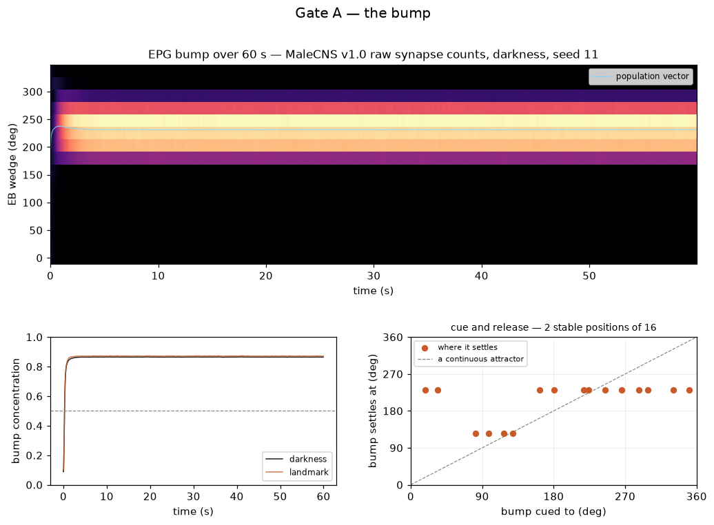
Seelig & Jayaraman 2015 (Nature 521:186-191) report that the EPG bump tracks heading with a stable offset under a visual landmark and that in darkness the offset accumulates error. This model reproduces the landmark case and does NOT reproduce the darkness drift: it is effectively pinned in both conditions (see caveats). No numeric drift rate is quoted from that paper because none was verified here.

What this does not show

• The attractor is discrete, not continuous. Cueing the bump into each of the 16 wedges and releasing it leaves 2 distinct settling positions at the operating point (see stable_positions_sweep for the gain dependence: it peaks at 6/16). The raw MaleCNS weights are not rotationally symmetric, and this model does not symmetrise them, because symmetrising is editing W.
• Consequently the dark-drift measurement is near zero and does not match Seelig & Jayaraman 2015. Reported, not fixed.
• The landmark is a tonic drive to the whole ER population, not an azimuth-resolved visual scene. An azimuth-resolved ER->EPG map is what SPEC 3.7's plasticity produces and is out of Gate A's scope.
• Gains are free parameters. Only the pathway structure and the signs are read from elsewhere (Hulse et al. 2021 architecture; MaleCNS neurotransmitter predictions).

Of the 4 outputs, 1 passes, 2 are partial and 1 fails: Tm20. A partial is a partial: it is not counted towards the passes anywhere on this page. Every verdict below is computed from the row above it by the rule stated here, not written out by hand.

An internal check that could have failed

The photoreceptor tuning peaks are MEASURED out of the running rate model, not read back from the opsin table. They should land on the Salcedo et al. 1999 lambda_max the curves were built from (for Rh1, its curve peak); any offset is the recurrent circuit (Dm9 feedback and the R7<->R8 axo-axonal inhibition) pulling the peak.

Rh1's curve peaks at 345 nm, not at its 478 nm lambda_max, because R1-R6 carry the 3-hydroxyretinol sensitising pigment. The curve published with Christenson et al. 2024 (rh1_standard.csv) peaks at 345 nm too. So R1-R6 is checked against its curve peak, and the lambda_max column is kept alongside so the difference is visible rather than hidden.

One qualification on “could have failed”, since it is the point of the check. Four of the five rows are measured against a λmax this model did not choose. R1–R6 is not: the 345 nm peak its curve is checked against is produced by the sensitising-pigment amplitude listed as a free parameter under the pigment table below. That row could still have failed — the recurrent circuit could have pulled the measured peak off the curve, as it did by 5 nm for R7y — but the curve it is checked against is partly ours.

Was the circuit actually being exercised

Is the circuit actually being exercised, or idling near its background? For every type, over the whole probe set: the rate range, how much of the total input is recurrent rather than the tonic background, and whether the cell is ever silenced (r = 0) or ever pinned at r_max. A circuit whose outputs never move more than a few percent off background is not reporting anything about hue and must not be read as if it were.

The fly paints what it sees, which changes what it sees. Whether that settles, oscillates or does something better was the first thing to find out. It settles: held still under a fixed illuminant, the loop is a contraction with one stable fixed point, and how quickly it gets there is a measurement rather than a sentence, so it is quoted below.

Read that as a statement about this loop. It uses the opaque reflectance, which returns the same colour however much paint is present, so it is a map on the pigment ratio alone and settling is the only thing it could have done — its second half figures below are exactly zero for that reason. The engine runs a finite layer over the paper, where the amount of paint is visible. What that is worth over a whole piece is the block after this one.

DULL, and measured to be dull rather than assumed. Every one of the four pigment orderings converges to a FIXED POINT within about two seconds. Second-half colour variance is 0.000000 for all four, and 0.000000 in all 25 cells of the deposition x renewal scan. The whole-run variance the SPEC §15 metric reports (0.06 to 0.32, RMS deltaE 0.24 to 0.56) is entirely the single transient from white paper to the equilibrium colour, and every one of those numbers is below deltaE 1, a just-noticeable difference. So the ordering chosen by the stated metric is chosen on the length of a transient, not on liveliness, and the choice should be read as close to arbitrary. All four numbers are recorded above so that is auditable. No noise was added to make this look otherwise (CLAUDE.md rule 4). Why, mechanistically: SPEC §3.4's loop, taken literally at one point on the canvas, is a contraction. More ink makes the patch darker, which lowers every photoreceptor's quantum catch; every photoreceptor in the dataset is histaminergic and therefore subtractive, so less catch means less inhibition downstream and slightly more ink. That is a monotone map with a single stable fixed point and no phase lag anywhere in it — the circuit's time constant (20 ms) is far shorter than the 100 ms tick, so each tick lands on the map's fixed point before the next one starts. There is nothing in the loop that could oscillate. What this means for the piece, stated for the engine rather than buried: colour variation in a finished piece will NOT come from temporal dynamics at a point. It has to come from the fly moving across a canvas that has history — crossing its own dried strokes, meeting wet paint of a different mix, and the illuminant changing with the real sky over the length of a piece. Those are all in the spec already (§3.3, §3.5, §6); none of them is in this gate, which deliberately holds the fly still under D65 to isolate the circuit. The honest headline is that the closed colour loop contributes a stable equilibrium colour, and the variation comes from the world and the walk.

All four orderings, so the choice is auditable

The metric, stated once

THE METRIC, stated once.

Colour variance over the run = the mean squared CIELAB distance of the
1 Hz samples of DEPOSITED INK from their own mean:

    V = (1/N) sum_i ||Lab_i - mean(Lab)||^2

which is the trace of the covariance of (L*, a*, b*). Its square root is an
RMS deltaE_ab from the run's mean colour, so it reads in familiar units.
Deposited ink, not accumulated canvas, because the canvas integrates and would
report a large variance for a run that simply drifts once and stops.

How far the colour actually moves over a piece

Measured on deposited ink sampled over a whole piece, as rms ΔE_ab from the run’s own mean, against 2.3 for a difference you could see. Across thirteen measurements — three seeds in the morning, at midday and in the afternoon, and four at night — it runs 1.26 to 1.37. So a piece is a wash that shifts, seen side by side, rather than one you would notice shifting, and that is printed rather than tuned away.

What is compressing it is which cells are in the model, not how far the fly walks. Tm5a and Tm5b swing across three-quarters of their range over a piece (0.725 and 0.761); Tm5c and Tm20 move 0.127 and 0.095 of theirs. Those are the two outputs the modelled patch is most missing the inputs of: 78% and 77% of the synapses reaching them in this dataset come from cells that are not in it.

Putting those cells in was tried, in full, and it made the painting worse. The fifteen tiling types that reach all seven columns took the colour circuit from 99 cells and 4,627 synapses to 205 and 21,704 and closed 55.8% of the missing input. Refitted, it scored 0.59498 on the hue-selectivity objective against 1.28282 — the best score ever measured — and the piece came out at rms ΔE 0.29 against 1.32. The reason is in the two stimuli: that objective is scored over sixty-one narrowband probes, and fitting it harder buys a cell that responds to fewer wavelengths, while a piece runs under a broadband illuminant where a more selective column produces four output rates that are more alike — and four alike concentrations mix to one colour. The wider roster was reverted. What would make it worth its cost is an objective scored under the light a piece actually runs in; that is the measurement below, and it is a new question rather than a bigger roster.

Where the engine no longer runs these numbers

The loop measured above is not the loop the engine runs, so two of its three canvas parameters have moved. The measured numbers stay published as measured. Every key where the engine differs is listed here, and a test asserts this list covers exactly the keys that differ, so a third divergence cannot appear without being written down.

The hue-selectivity measurement above has to use the stimulus the published paper used: sixty-one narrowband probes. That is the right instrument for that question and the wrong one for any other — the block above records what happened when it was used as one. This is the same question asked under the light and the paint a piece actually has.

A stimulus here is a pair: light and paint, both computed the way the piece computes them — the sky model plus the practical lamp below its threshold, and the finite paint layer over the paper rather than the opaque one. Both are held to the engine’s own code at 1e-12 by a test, so “the light the piece runs in” is a checked claim rather than an intention. Nothing here is fitted: there is no published target to fit to, and fitting gains until a piece had more colour in it would be tuning away a dull measurement. What it is for is rejecting a circuit that scores well on narrowband probes by going blind under daylight.

What each output does under this light

This is the row that matters, and it is the one no narrowband probe could show. Two of the four outputs barely move across the whole ensemble, so two of the four pigments are close to a constant and the mixture the fly can reach is close to a line rather than a volume. That is a fact about this roster measured against this light; it is not a verdict on the connectome, and it is not being corrected here.

The floor’s job is to reject the collapse the wider roster produced. Setting it honestly needed this measurement on that circuit as well as on this one, so that circuit was rebuilt outside the tree and both ends are measured on the same ensemble by the same code:

The floor is the geometric mean of those two separations, which puts the published circuit exactly as far above it in ratio as the collapse is below it — 1.375× either way. A geometric mean rather than an arithmetic one because separation is a coefficient of variation, so the halfway point between two of them is multiplicative. That rule is the whole of the choice.

It is a constraint and never a term. The gain fit still optimises the published numbers and nothing else; this only refuses candidates below the floor. No gain is moved in order to raise a colour range — that would be tuning away a measured dullness. Re-running the fit with the constraint switched on returns the published table unchanged, to five decimal places, at loss 1.28284 against 1.28282: it does not bind here, and it would have rejected the collapse.

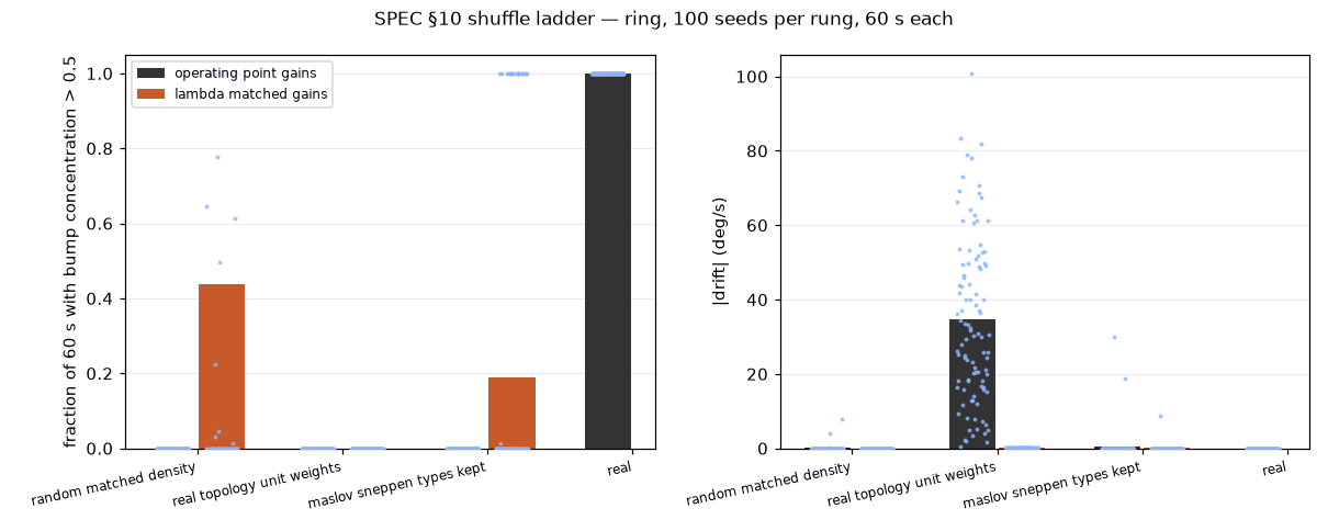
Four rungs in increasing strength — a random graph at matched density, the real topology with unit weights, a degree-preserving shuffle with cell types kept, and the real matrix. Gains, signs, type labels, inputs and probes are held fixed across the rungs, so the only thing that changes is the wiring.

Ring

fraction of a 60 s run with EPG bump concentration > 0.5; drift = |least-squares slope of unwrapped heading|, deg/s

The ladder as designed: 100 seeds per rung, 60 s each, seed 4242. All 4 rungs completed at that count, in every gain setting each was run in. Real network leading eigenvalue: 1.7358. Every rung, with its numbers.

What the measured rungs do and do not show

The number to be careful with is the random rung with its gains rescaled to λ_max. It holds a bump — concentration above 0.5 for more than half the run — in 44 of 100 seeds, and read alone that looks like the control half working. The spread says otherwise. Across those 100 seeds the fraction of the run spent above 0.5 has mean 0.438 and standard deviation 0.484, against 0.496: the largest standard deviation any quantity bounded between 0 and 1 with that mean can have, which is reached only by a quantity that is always exactly 0 or exactly 1. The measured spread is 97.5% of that bound and the maximum is 1.000, so the seeds sit at the two ends and not in the middle. A rescaled random graph either localises for essentially the whole run or for essentially none of it. It is bimodal, not partial.

That is why the concentration metric is stated as narrowly as it is. Concentration above 0.5 measures localisation — activity gathered into one place on the ring rather than smeared around it — and enough recurrent gain will localise a random graph. It does not measure a heading map. Nothing in it ties where the activity sits to where the fly is pointing, and the drift column does not fill the gap: a lump of activity that sits still because nothing is moving it has as little drift as one held in place by a landmark, which is what 0.0055 °/s on the rescaled random rung against 0.0012 °/s on the real matrix is showing. So the honest reading of this rung is the narrow one: rescaled recurrent gain buys localisation on some seeds and nothing else the ladder can see. The rescaling is the steel-man — the control is handed the same amount of recurrent gain as the real network and still has to produce the behaviour out of its own topology.

This is one circuit and one computation — a heading representation in the ellipsoid body and protocerebral bridge of one fly. It is not a claim about the brain.

Colour column

hue-selectivity index (lifetime sparseness) per output type

What the ladder shows

MIXED, and the mix is the interesting part. A random graph at matched density destroys hue selectivity completely (0.21-0.23 across all four outputs, against 0.35-0.77 real) - so the selectivity is not an artefact of the gains, the signs or the input. But the SPEC §10 degree-preserving shuffle WITH TYPES KEPT does not collapse it: it retains 82-107% of the real index. Lifting the type restriction collapses it to 0.26-0.29, i.e. to the random-graph level. Read plainly: in this 99-cell patch the selectivity is carried by the TYPE-LEVEL connectivity read from the connectome - which type contacts which type, and how heavily - and not by which individual cell contacts which individual cell. A same-type-preserving swap leaves the type-by-type weight matrix intact, so there is nothing left for it to destroy. The live 'shuffle wiring' toggle on the page must therefore use the types-free shuffle, or the random rung, and say which. Every number in this paragraph is read out of `results` above rather than typed: they were typed once, and the roster change of 2026-09-16 made all of them wrong at once while the page went on printing them.

100 seeds, 10 swaps per edge, seed 20260915. Held fixed: gains, signs, type labels, inputs, integrator, probe set. Every rung, and the diagnostic rung, with its numbers.

This circuit, this computation. Not the whole brain, and not a claim that shuffling any connectome destroys any function.

The one aesthetic decision in the project, and the only lever on the colour loop. Each hue-selective output drives one pigment; the four concentrations mix under Kubelka–Munk.

What the pigment data is not

• No public dataset of SEPARATE Kubelka-Munk K and S for named artist pigments exists. Berns 2016/2019 and Berns 2022 measured exactly that for PV19, PB29 and PG7; neither spreadsheet is downloadable (the 2022 one has been withdrawn by its author) and Okumura 2005 publishes its unit k and s as graphs only. So this is masstone reflectance turned into SINGLE-constant K/S, not two-constant Kubelka-Munk.
• UV, and this is the SPEC §13 'UV is a translation' caveat made specific: PY3 and PV19 are measured from 291 nm, so their 300-400 nm reflectance is real data. PB29 and PG7 are measured only from 360.2 nm; from 300 to 360 nm their value is HELD CONSTANT at the 360.2 nm reading, which is an assumption, not a measurement. Rh3 (345 nm) and Rh4 (375 nm) both sit in or next to that gap, so two of the fly's five channels are reading partly-assumed numbers off two of the four pigments.
• PG7: the source file is named only 'phthalo green' and carries no Colour Index number. The same archive family labels PG36 separately, so PG7 is a strong inference, not a reading. Its masstone is near-black (R 6.7-11% across the visible), the classic single-constant failure case: K/S comes out flat and noise-dominated.
• PV19 here is the violet (beta) polymorph; SPEC §6 names quinacridone rose, which is the rose/gamma form and has a different spectrum.
• Masstone films of transparent organics (PV19, PG7) may not be optically thick, which violates the opaque-layer assumption behind the inversion.

The opsins the ink is computed through are published measurements with one free parameter inside them. The peak sensitivities are not a choice; the curve shape is a published template evaluated at them; and the sensitising pigment carried by R1–R6 has an amplitude that is ours.

Salcedo et al. 1999, J Neurosci 19(24):10716-10726. Curve shape: Govardovskii et al. 2000, eqs. 1-5 (alpha + beta band).

How each curve was built, quoted rather than summarised

Salcedo et al. 1999 (J Neurosci 19:10716-10726) publish lambda_max for the Drosophila rhodopsins but not digitised sensitivity curves, so each curve here is the A1 visual-pigment template of Govardovskii, Fyhrquist, Reuter, Kuzmin & Donner 2000 (Visual Neuroscience 17:509-528), alpha band plus beta band, evaluated at the published lambda_max and normalised to a peak of 1. Nothing is hand-drawn. R1-R6 additionally carry the 3-hydroxyretinol sensitising pigment (Kirschfeld et al. 1977), added to Rh1 as a Gaussian antenna band at 350 nm; its relative amplitude is a FREE parameter, listed below.

The free parameter inside the opsins

visible_to_uv_ratio is the free one, and it is not a small detail of the curve: at 0.526 the antenna band exceeds Rh1’s own 478 nm λmax, so the R1–R6 sensitivity curve peaks at 345 nm instead. That is the curve the internal check above measures R1–R6 against, and the note under that check says so.

Every measurement above was made in Python. Everything you can watch on the studio page is computed in TypeScript. Those are two implementations of one rate equation, and if they have drifted apart then the proof on this page is proof of something the site does not run.

The reference writes a fixture out of the same code path that produced the heading measurement; the engine rebuilds the same quantities from its own circuit and is compared against it, so a disagreement implicates the engine rather than the fixture. The fixture is published with the rest of the results files, and everything below is counted out of it.

One thing is deliberately not compared: the noise term, which is zero on both sides of the fixture. Parity fixture for engine/parity.test.ts. Noise is zero by design; see the module docstring in prep/parity.py for why, and engine/rng.test.ts for the generator's own tests. The two implementations draw from different generators — splitmix64 with Box–Muller on one side, xoshiro128** on the other — so their noise streams cannot agree sample for sample, and porting one to the other language purely to satisfy a test would prove nothing about the model. What is compared is the part that could be wrong in a way nobody would notice: the effective matrix, the sparse accumulation, the rectifying nonlinearity and the Euler step. The generator has its own determinism and distribution tests, and so does the replay guarantee that makes a piece reproducible from its seed.